Standard_Normal_Distribution.png

Size of this preview:
800 × 494 pixels
.
Other resolutions:
320 × 198 pixels
|
640 × 396 pixels
|
1,024 × 633 pixels
|
1,280 × 791 pixels
|
2,560 × 1,582 pixels
|
5,986 × 3,700 pixels
.

|
This
math
image could be re-created
using
vector graphics
as an
SVG
file
. This has several advantages; see
Commons:Media for cleanup
for more information. If an SVG form of this image is available, please upload it and afterwards replace this template with
{{

vector version available

|

new image name

}}
.
It is recommended to name the SVG file “Standard Normal Distribution.svg”—then the template Vector version available (or Vva ) does not need the new image name parameter. |
Summary
| Description |
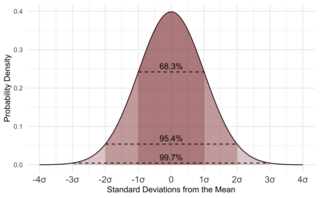
English:
The Standard Normal Probability Distribution with shaded regions
|
| Date | |
| Source | Own work |
| Author | D Wells |
| Other versions |
[
]
|


<code><code><code><languages/></code></code></code>
Licensing
I, the copyright holder of this work, hereby publish it under the following license:
This file is licensed under the
Creative Commons
Attribution-Share Alike 4.0 International
license.
-
You are free:
- to share – to copy, distribute and transmit the work
- to remix – to adapt the work
-
Under the following conditions:
- attribution – You must give appropriate credit, provide a link to the license, and indicate if changes were made. You may do so in any reasonable manner, but not in any way that suggests the licensor endorses you or your use.
- share alike – If you remix, transform, or build upon the material, you must distribute your contributions under the same or compatible license as the original.
Source code
library(ggplot2)
p <- ggplot(NULL, aes(c(-4,4))) +
  geom_line(stat = "function", fun = dnorm) +
  geom_area(stat = "function", fun = dnorm, fill = scales::muted("blue"), xlim=c(-1,1), alpha=1/4) +
  geom_area(stat = "function", fun = dnorm, fill = scales::muted("blue"), xlim=c(-2,2), alpha=1/4) +
  geom_area(stat = "function", fun = dnorm, fill = scales::muted("blue"), xlim=c(-3,3), alpha=1/4) +
  theme_minimal() +
  theme(axis.text.x = element_text(size = 12)) +
  scale_x_continuous(labels = label_units, breaks = -4:4) +
  xlab("Standard Deviations from the Mean") +
  ylab("Probability Density") +
  geom_segment(aes(x=-1, xend=1, y=dnorm(1), yend=dnorm(1)), linetype="dashed") +
  geom_segment(aes(x=-2, xend=2, y=dnorm(2), yend=dnorm(2)), linetype="dashed") +
  geom_segment(aes(x=-3, xend=3, y=dnorm(3), yend=dnorm(3)), linetype="dashed") +
  annotate("text", x = 0, y = dnorm(1)+0.015, label = "68.3%") + #pnorm(1)-pnorm(-1) %
  annotate("text", x = 0, y = dnorm(2)+0.015, label = "95.4%") +
  annotate("text", x = 0, y = dnorm(3)+0.015, label = "99.7%")

ggsave("Normal_Distribution.png", p, width = 3.7*1.618, height = 3.7, dpi = 1000)